Computation Boot Camp
Day 3 Unsupervised Analysis
Principal Component Analysis (PCA)
- For data exploration and visualization
- Reduce the dimendionality of large data set
- Maintain structure of the data
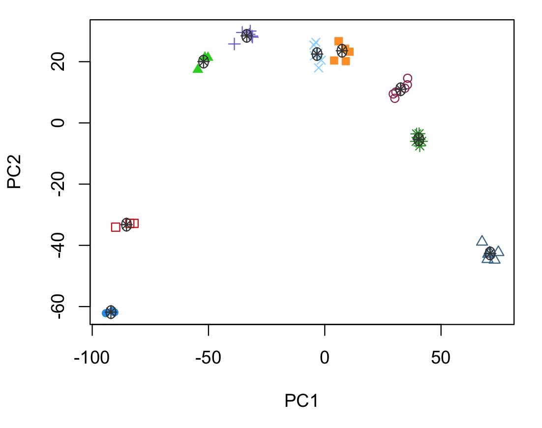
Developmental trajectory of murine cardiomyocytes
PCA -- how does it work?
Input: matrix where rows are variables and columns are entities (e.g. rows=genes, columns=samples).
Computation: Iteratively search for loadings that maximize the variance (var = average of the squared differences from mean)
Outputs:
(A) Loadings matrix of the normalized contribution of a gene to a PC
- columns correspond to 1st, 2nd, 3rd, ..., PCs
- rows correspond to genes
(B) Scores matrix
- columns correspond to samples
- rows correspond to PC
How to do this in R?
Fetch code and data from website.
- Code: http://cahanlab.org/intra/training/bootcampJune2016/misc/utils.R
- Data 1: http://cahanlab.org/intra/training/bootcampJune2016/misc/expDat.R
- Data 2: http://cahanlab.org/intra/training/bootcampJune2016/misc/sampTab.R
Launch R, load data. Alter paths below for your setup ...
source("../../misc/utils.R")
library(ggplot2)
expRun<-utils_loadObject("../../misc/expDat.R")
stRun<-utils_loadObject("../../misc/sampTab.R")
Take a look at the data
dim(expRun)
## [1] 2000 1000
expRun[1:3,1:3]
##          GSM501434 GSM287580 GSM287575
## Copg1     5.848932  5.569252  5.615026
## Atp6v0d1  7.841972  8.928719  8.832163
## Golga7    8.573669  8.924030  8.908230
Take a look at the data
dim(stRun)
## [1] 1000 10
stRun[1:3,c(2,3,4,10)]
##           sample_id                                            sample_name
## GSM501434 GSM501434 LX_ND_10_36_9_CH12LX_T_1_111908_Mouse430_2_RSTMSU601_9
## GSM287580 GSM287580            Memory Tx B cell (FG)_2nd generation screen
## GSM287575 GSM287575          Naive AA4.1- B cell (A)_2nd generation screen
##           description1 description6
## GSM501434        bcell        blood
## GSM287580        bcell        blood
## GSM287575        bcell        blood
Run PCA
system.time(xFF2<-prcomp(t(expRun), center=T, scale=T))
##    user  system elapsed
##   7.328   0.087   7.421
Glimpse at the results
class(xFF2)
## [1] "prcomp"
names(xFF2)
## [1] "sdev" "rotation" "center" "scale" "x"
dim(xFF2$rotation) # loadings
## [1] 2000 1000
dim(xFF2$x) # scores
## [1] 1000 1000
How much total variation does each PC explain?
pcaVals2<-xFF2$x
pcaVals2<-data.frame(pcaVals2);
pcaVals2<-cbind(pcaVals2, stRun) # don't worry about this now...
varExpl2<-xFF2$sdev**2 / sum(xFF2$sdev**2)
varExpl2[1:5]
## [1] 0.14946926 0.08713941 0.06243711 0.06170882 0.05702081
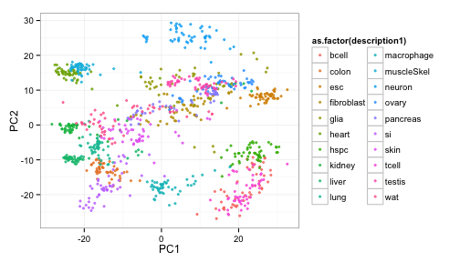
Finally, plot the results, color by cell type
ggplot(pcaVals2, aes(x=PC1, y=PC2, colour=as.factor(description1)) ) +
geom_point(pch=19, alpha=3/4, size=1) +
theme_bw() +
guides(colour=guide_legend(ncol=2))
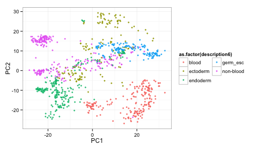
Plot the results, color by germ layer descended from
ggplot(pcaVals2, aes(x=PC1, y=PC2, colour=as.factor(description6)) ) +
geom_point(pch=19, alpha=3/4, size=1) +
theme_bw() +
guides(colour=guide_legend(ncol=2))
What genes contribute most to the PCs?
g1<-names(sort(abs(xFF2$rotation[,1]), decreasing=T)[1:25])
g2<-names(sort(abs(xFF2$rotation[,2]), decreasing=T)[1:25])
g1[1:4]
## [1] "Cct2" "Cct5" "Rbm12" "S100a1"
g2[1:4]
## [1] "Elf1" "Ikbke" "Ifi47" "Kifap3"
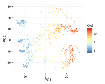
Overlay the expression of these genes on PCA plots
library(RColorBrewer)
ColorRamp <- colorRampPalette(rev(brewer.pal(n = 7,name = "RdYlBu")))(100)
pcaVals2<-cbind(pcaVals2, t(expRun))

ggplot(pcaVals2, aes(x=PC1, y=PC2, colour=Cct2) ) +
geom_point(pch=19, alpha=3/4, size=1) +
theme_bw() +
scale_colour_gradientn(colours=ColorRamp)
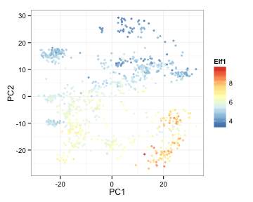
Overlay the expression of these genes on PCA plots
library(RColorBrewer)
ColorRamp <- colorRampPalette(rev(brewer.pal(n = 7,name = "RdYlBu")))(100)
pcaVals2<-cbind(pcaVals2, t(expRun))

ggplot(pcaVals2, aes(x=PC1, y=PC2, colour=Elf1) ) +
geom_point(pch=19, alpha=3/4, size=1) +
theme_bw() +
scale_colour_gradientn(colours=ColorRamp)
Assignment
Single cell expression data described here: http://software.10xgenomics.com/files/samples/cell/pbmc3k
- Download pre-cleaned single cell expression data from: http://www.cahanlab.org/intra/training/bootcampJune2016/misc/expSingleCell.R
- Load this data into R
- Run PCA on it
- How much variation is explained by the 1st 5 components?
- Plot the first two PCs using ggplot2
- What genes contribute most to each of the first 2 PCs?
- Use ggplot2 to overlay expression of the top gene for each PC onto the PCA plot