
Computation Boot Camp
Patrick Cahan
Objectives
- Nudge you towards proficiency and comfort with big data analysis
- Develop culture of 'soups-to-nuts' reproducibility in our analytics
Course website: http://cahanlab.org/intra/training/bootcampJune2016/
Course schedule
- Monday: Intro to R and making simple, pretty presentations
- Tuesday: Data wrangling
- Wednesday: Unsupervised analysis
- Thursday: Supervised analsyis
- Friday: wrap up
Daily schedule
- Morning: Background to topic, tutorials
- Break: lunch, do what you need to do
- Afternoon: Work on assignment (individually) that you will present the following morning
Inspiration and resources for this course
- Andrew Jaffe's short course: http://aejaffe.com/winterR_2016/
- R cookbook: http://www.cookbook-r.com/
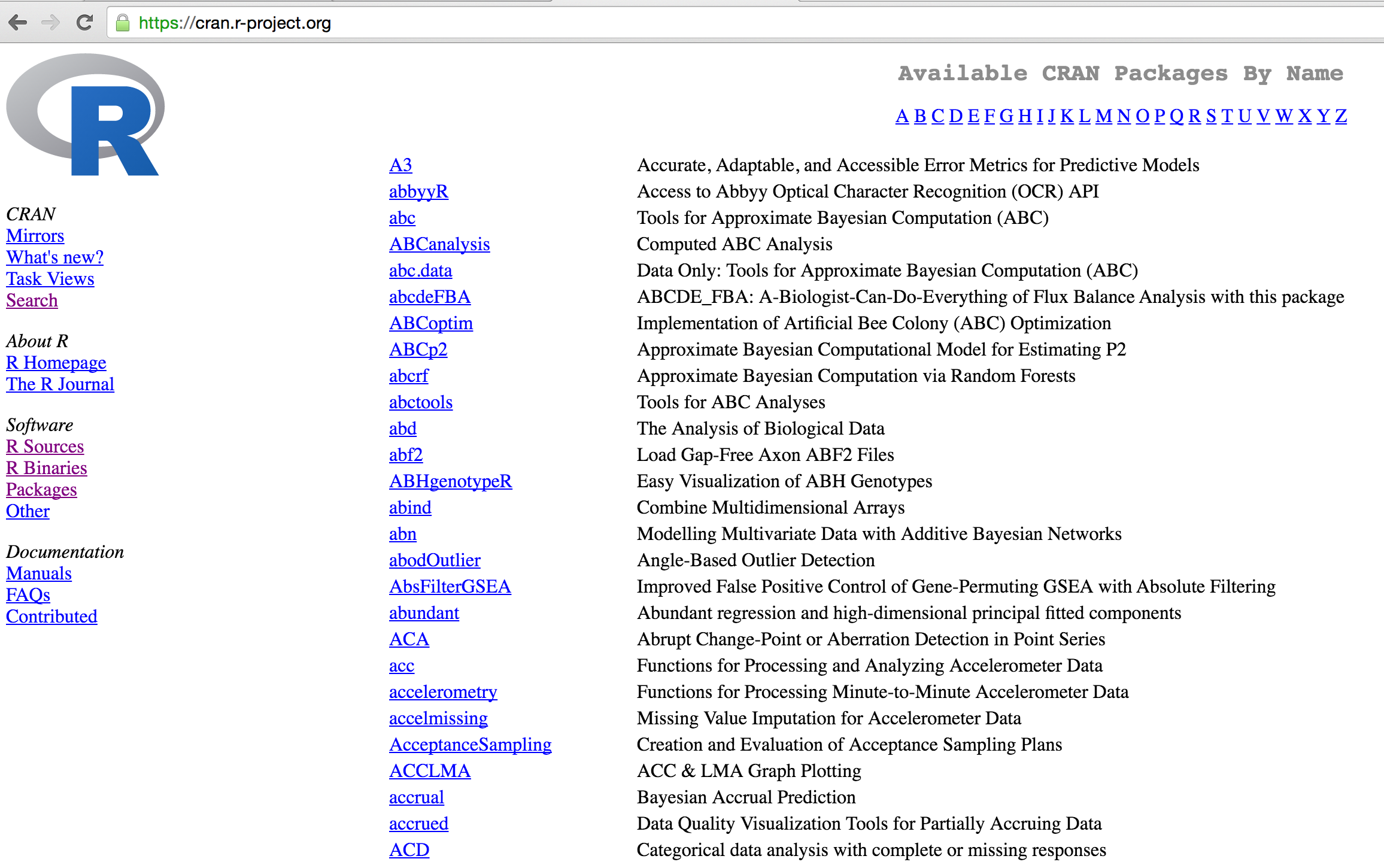
- R and R packages: https://cran.r-project.org/
- Color palettes: http://colorbrewer2.org/
- R Markdown: http://rmarkdown.rstudio.com/index.html
- Embedding R code into presentations: http://zevross.com/blog/2014/11/19/creating-elegant-html-presentations-that-feature-r-code/
- Embedding R into presentations: http://ramnathv.github.io/slidifyExamples/
- Embedding R into presentations: https://www.uvm.edu/rsenr/vtcfwru/R/fledglings/14_Slideshows.html
- Git and GitHub: http://readwrite.com/2013/09/30/understanding-github-a-journey-for-beginners-part-1/
- R reference card: http://cran.r-project.org/doc/contrib/Short-refcard.pdf
- Online interactive exercise: http://tryr.codeschool.com/
- Free and excellent text editor with R syntax highlighting: http://www.sublimetext.com/2
What is R?
- R is a language and environment for statistical computing and graphics
- There are hundreds of user-contributed packages
- Interpreted, not compiled
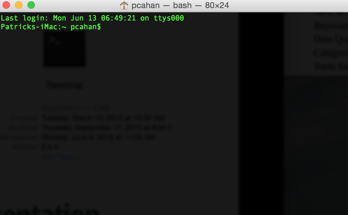
Launch R from your Terminal
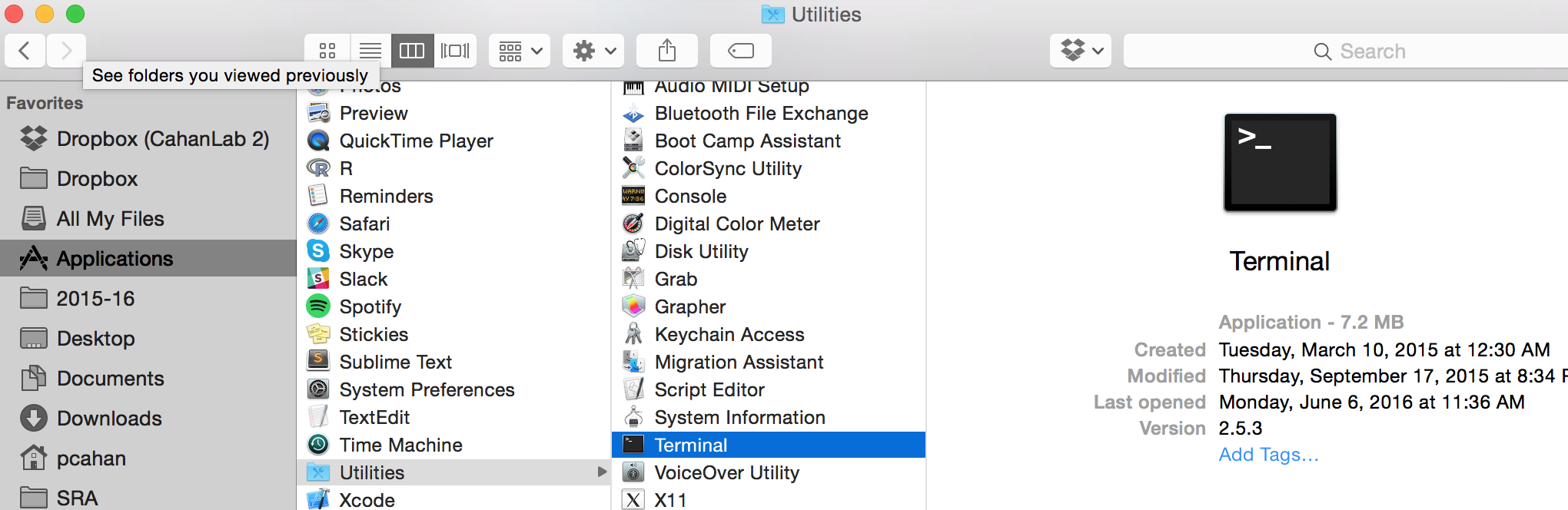
Meet your new friend, Terminal
Basic interactions with the shell
List the contexts of your current working directory
ls -laht
Make a new directory, or folder, and 'go there':
mkdir ~/bootcamp2016/
cd ~/bootcamp2016
mkdir day1
cd day1
Now launch R
R
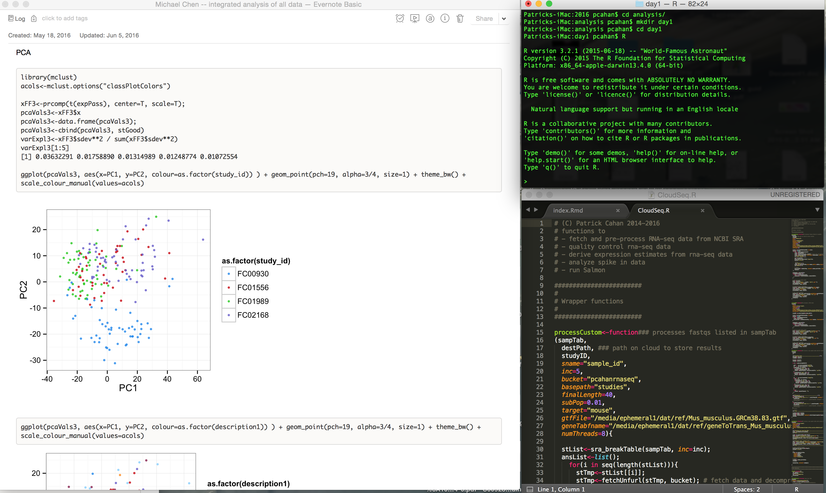
How I interact with R
- Evernote for writing code, then cut and paste into terminal.
- Text editor (Sublime 2) for writing functions
How this all works
In slides, a command (we'll also call them code or a code chunk) will look like this
print("I'm code")
## [1] "I'm code"
And then directly after it, will be the output of the code. So print("I'm code") is the code chunk and [1] "I'm code" is the output.
R is a calculator
2 + (2 * 3)^2
## [1] 38
(1 + 3) / 2 + 45
## [1] 47
Sequences and functions
1:10
## [1] 1 2 3 4 5 6 7 8 9 10
1:10 is equivalent to the seq function
seq(from=1,to=10,by=1)
## [1] 1 2 3 4 5 6 7 8 9 10
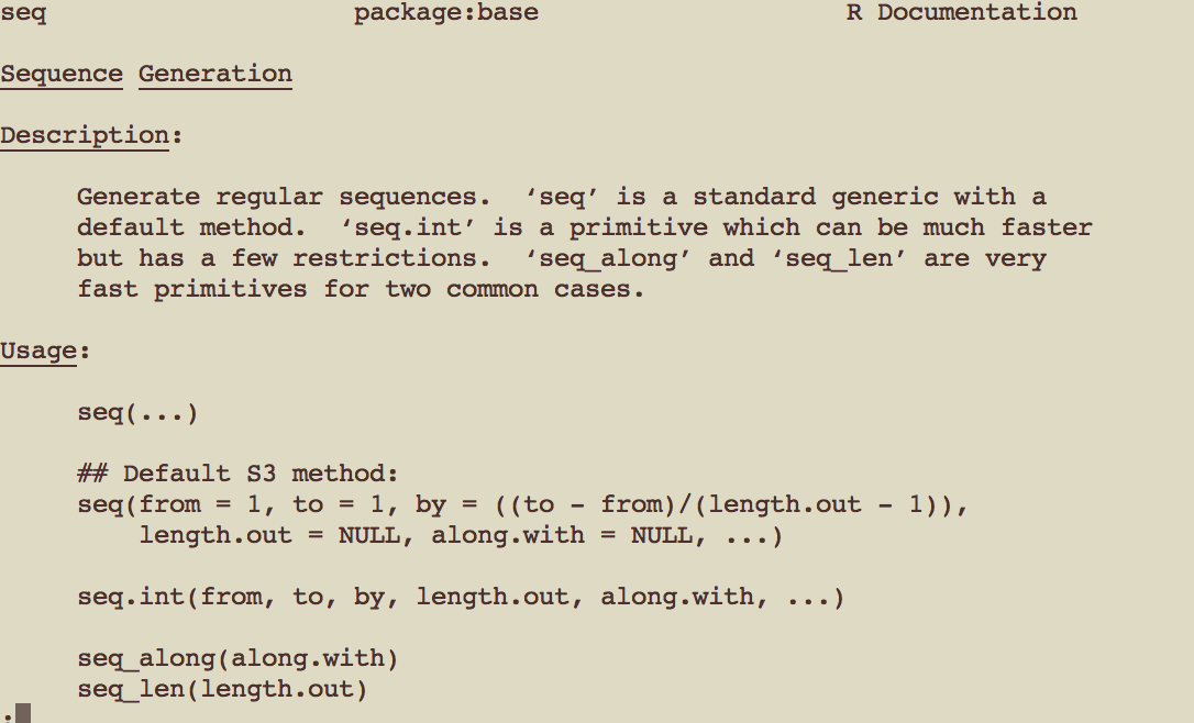
Help
To learn more about a function, use help
?seq
Variables
Most of the time you want to capture the results of a computation. Variables
- Create variables from within the R environment and from files on your computer
- Use "=" or "<-" to assign values to a variable name
- Case-sensitive
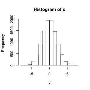
x <- rnorm(1e4, mean=0, sd=2) # result does not get sent to output
R's listing function, ls:
ls()
## [1] "x"
Variables and a bit of plotting
Things can be done with variables
mean(x);
## [1] 0.03374283
hist(x);

Variable classes
- Classes define the structure of a variable, and the set of operations or functions that can performed on them
- vector and matrix are classes
- data.frame is one of the most frequently used classes of R variables
- data.frame is like a spreadsheet. Rows are entities and columns are variables characterizing that entity.
data.frames are somewhat advanced objects in R
Here we introduce "1 dimensional" classes; these are often referred to as 'vectors'
Vectors can have multiple sets of observations, but each observation has to be the same class
class(x)
## [1] "numeric"
y = "mistakenly, embryomics, smoogy boogy"
print(y)
## [1] "mistakenly, embryomics, smoogy boogy"
class(y)
## [1] "character"
combine (C)
The function c() collects/combines/joins single R objects into a vector of R objects. It is mostly used for creating vectors of numbers, character strings, and other data types.
x <- c(1, 4, 6, 8)
x
## [1] 1 4 6 8
class(x)
## [1] "numeric"
Length ...
length(): Get or set the length of vectors (including lists) and factors, and of any other R object for which a method has been defined.
length(x)
## [1] 4
y
## [1] "mistakenly, embryomics, smoogy boogy"
length(y)
## [1] 1
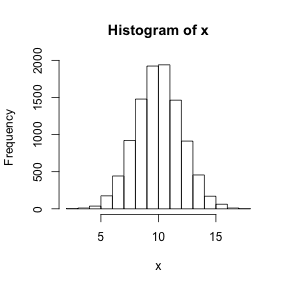
Operating on vectors
x <- rnorm(1e4, mean=0, sd=2)
hist(x)
x <- x + 10
hist(x)
Let's try this out...
Go to http://tryr.codeschool.com/ and earn your chapter badges!

Each row represents one character from the book series Game of Thrones
Download data from http://www.cahanlab.org/intra/training/bootcampJune2016/misc/character-deaths.csv
Load the data, modify path accordingly...
survdata<-read.csv("../../resources/character-deaths.csv", as.is=TRUE)
dim(survdata)
## [1] 917 13
colnames(survdata)
##  [1] "Name"               "Allegiances"        "Death.Year"
##  [4] "Book.of.Death"      "Death.Chapter"      "Book.Intro.Chapter"
##  [7] "Gender"             "Nobility"           "GoT"
## [10] "CoK"                "SoS"                "FfC"
## [13] "DwD"
ggplots2: http://ggplot2.org/
Use ggplot2 to make nice graphics
Install the package if you don't already have it...
install.packages("ggplot2")
Load the library
library(ggplot2)
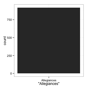
take a look at the data
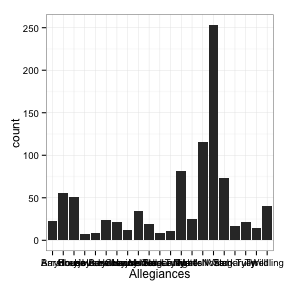
How many characters per house?
ggplot(survdata, aes(x="Allegiances")) + geom_bar(stat="bin") + theme_bw()
take a look at the data -- Take II
How many characters per house?
ggplot(survdata, aes(x=Allegiances)) + geom_bar(stat="bin") + theme_bw()
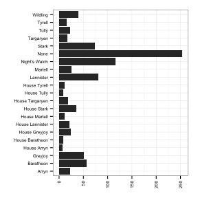
take a look at the data -- Take III
How many characters per house?
ggplot(survdata, aes(x=Allegiances)) + geom_bar(stat="bin") + theme_bw() + theme(text = element_text(size=8), axis.text.x = element_text(angle=90, vjust=0.5, hjust=1)) +
    theme(axis.title.x = element_blank())+ ylab("") + xlab("") + coord_flip()
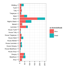
Dead/Alive
length(which(is.na(survdata$Death.Year)))
## [1] 612
length(which(!is.na(survdata$Death.Year)))
## [1] 305
Dead/Alive
isDead<-rep("Dead", nrow(survdata))
isDead[ which( is.na(survdata$Death.Year)) ] <-"Alive"
survdata<-cbind(survdata, isDead=isDead)
ggplot(survdata, aes(x=Allegiances, fill=as.factor(isDead))) + geom_bar(stat="bin") + theme_bw() + theme(text = element_text(size=8), axis.text.x = element_text(angle=90, vjust=0.5, hjust=1)) +
    theme(axis.title.x = element_blank())+ ylab("") + xlab("") + coord_flip()
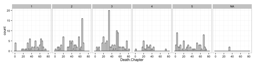
When do most characters die?
ggplot(survdata, aes(x=Death.Chapter)) + geom_histogram(colour="black", fill="white") + facet_grid(. ~ Book.of.Death) + theme_bw()
## stat_bin: binwidth defaulted to range/30. Use 'binwidth = x' to adjust this.
## stat_bin: binwidth defaulted to range/30. Use 'binwidth = x' to adjust this.
## stat_bin: binwidth defaulted to range/30. Use 'binwidth = x' to adjust this.
## stat_bin: binwidth defaulted to range/30. Use 'binwidth = x' to adjust this.
## stat_bin: binwidth defaulted to range/30. Use 'binwidth = x' to adjust this.
## stat_bin: binwidth defaulted to range/30. Use 'binwidth = x' to adjust this.
World university rankinks from: https://www.kaggle.com/mylesoneill/world-university-rankings/version/2
Download from http://www.cahanlab.org/intra/training/bootcampJune2016/misc/timesData.csv
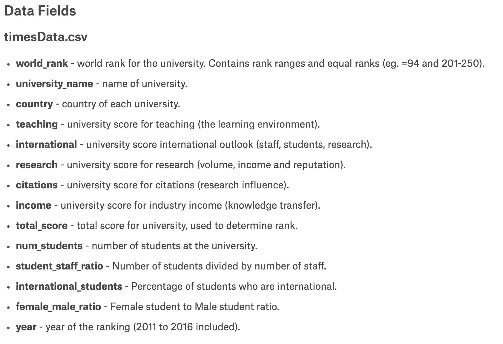
Your assignment, ussing ggplot2...
- Use facets to plot distributions of teaching scores, one plot per year
- Scatter plot to explore relationship between the teaching score and the income (facet by year)
- Add a regression line to the above plot
- Same as 2 and 3 but exploring the relationship between total_score and income
- Same as 2 and 3 but exploring relationship between world_rank and research
- Does there appear to be an effect of female_male_ratio and total_score? Use boxplot to visualize